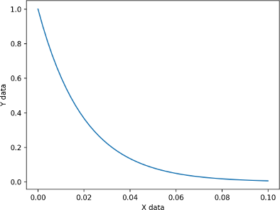
Non-linear curve fitting (or non-linear parametric regression)is a fundamental part of the quantitative analysis performed in multiple scientific disciplines. The main idea is that we know (or assume) the model that describes an observed data. For example, it would seem reasonable to assume that the curve below is described by an exponential decay function of the form $$ S= a * e^{(-xdata/b)} $$.

But, how do we test that this assumption is correct and estimate a and b ?. We find the values for a and b that minimize the square of the residuals between the predicted data assuming the exponential model and the observed data. In the next section I present a python code to perform non-linear curve fitting on a simulated curve.
# Objective
# Use non-linear curve fitting to estimate the relaxation rate of an exponential
# decaying signal.

# Steps
# 1. Simulate data (instead of collecting data)
# 2. Define the objective function for the least squares algorithm
# 3. Perform curve fitting
# 4. Compare results

# modules
import numpy as np
import matplotlib.pyplot as plt
from   scipy import optimize
# 1. Simulate some data
# In the real worls we would collect some data, but we can use simulated data
# to make sure that our fitting routine works and recovers the parameters used
# to simulate the data
def exp_decay(parameters,xdata):
    '''
    Calculate an exponetial decay of the form:
    S= a * exp(-xdata/b)
    '''
    a = parameters[0]
    b = parameters[1]
    return a * np.exp(-xdata/b)

xdata = np.linspace(0,.1,20)
A = 1.0
B = .050
parameters_used = [A,B]
y_data = exp_decay(parameters_used,xdata)

# Add Gaussian noise with mean = 0, and std. dev = 0.05
y_data_with_noise = y_data + np.random.normal(0,.05,(len(y_data)))

# Plot the simulated data
plt.plot(xdata,y_data_with_noise,'o',xdata,y_data,'-')
plt.legend(('Clean','With Noise'))

# 2. Define the objective function for the least squares algorithm
# The scipy.optimize.least_square requires the following inputs

# A) Objective function that computes the residuals of the
#     predicted data vs the observed data using the following syntaxis:
#     f = fun(parameters, *args, **kwargs),

def residuals(parameters,x_data,y_observed,func):
    '''
    Compute residuals of y_predicted - y_observed
    where:
    y_predicted = func(parameters,x_data)
    '''
    return func(parameters,x_data) - y_observed

# 3. Perform curve fitting
#    Initial guess for the parameters to be estimated
#    The parameters follow the same order than exp_decay
x0 = [1, 1]

#    Lower and uppers bounds
lb = [0,0]
ub = [2,2]

# estimate parameters in exp_decay
OptimizeResult  = optimize.least_squares(residuals,  x0, bounds = (0,2),
                                          args   = ( xdata, y_data_with_noise,exp_decay) )
parameters_estimated = OptimizeResult.x

# Estimate data based on the solution found
y_data_predicted = exp_decay(parameters_estimated,xdata)

# Plot all together
plt.figure(2)
plt.plot(xdata,y_data_with_noise,'ob',
         xdata,y_data           ,'--k',
         xdata,y_data_predicted ,'xr')
plt.legend(('Data With noise','Real Data','Predicted Data'))

# How good are the parameters I estimated?
print( 'Predicted: ' + str( parameters_estimated))
print( 'Expected : ' + str( parameters_used))
I am data scientist scientist, passionate about helping people using mathematics, programming and chemistry
